
In this Excel tutorial, we’ll go through a newer advanced function in Excel known as Dynamic Arrays. It’s a function that will revolutionize the way you use Excel by allowing you to efficiently handle complex data and generate dynamic results using a single formula.
Transcription
0:07 – 0:32 Hi everyone in this video we’re going over advanced Excel functions and in particular dynamic arrays. So recent versions of Excel, including Office 365 and Microsoft 365 have introduced some new functions that now allow you to work with dynamic arrays. These are basically tabular kinds of data as you see here, and it allows you to manipulate with a single formula a lot of information and create some dynamic results.
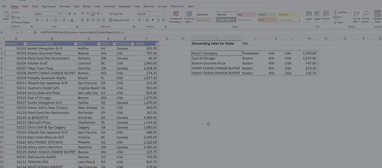
0:33 – 1:27 So we’re gonna use this particular tutorial to discuss three of these formulae and we’re already seeing the results of some of them on the right hand side, but I’m gonna quickly show you what the results look like and they’re going to deconstruct the formula that makes some work. So as you can see here on the left side, there’s a table of information that includes 1 line for each invoice with the customer name, the city, the state, the country (etc). But what we have on the right-hand side are what looks like manual extracts from there that first of all give U.S. sales and descending dollar values for any specified state. In this case it’s Massachusetts and they also show us each city into which we’ve sold anything. So I guess you know, one line per city and a unique list of cities that are included in this data. But you know, here’s the thing, these are dynamic arrays. So I’ll show you that in two ways.
1:27 – 1:56 Firstly, you can change the state that I’m looking at. So let’s just say I wanna look at, I don’t know, Alberta. Type in AB, it updates that first list immediately. And you know, say we wanna look at Ontario, we’ll get an updated list of Ontario. And if we go back to looking at say Massachusetts, which seems to have a few more, you know now we’re seeing the sales. So you’ll notice in each case the sales were sorted in descending dollar of selling order of dollar value.
1:57 – 3:05 The second thing is that both these will update in real time as we add or change data. So for example, if I decide that I’m going to relocate you know Concord out of Massachusetts and any New York, I just moved into town. You’ll notice that the descending Sales for state date has changed in real-time, so I’m gonna do that and put it back because that’s where it really belongs also if I add a new entry here, let’s just say our manually add. Uh, you know Clark’s company for example, and just say it’s Marks Company in Tinseltown, New York. You know, I can make this Massachusetts as well. And as I’m typing those varies on the right hand side are updating. And if I put this at like 3000 for example. Which is one of the top of the list and they’re dead. So I’m updating these arrays in real-time, which is super useful and you might wonder how I did this, but I took advantage of 3 formulae, and we’ll get to that in a minute.
3:08 – 3:52 So there are three formulae that we’re talking about. The first one is the filter formula, the second is the unique formula and the third is the sort formula. So the sort formula is actually one that I’m using around both the filter and unique formula to get the sort order that I want. The sort can be used on its own to sort of a copy of your source. Media any sort format or any sort order that you like. OK, so I’ve gotten rid of the formula that had for our descending sales by state and now I’m going to reinstate that formula so I can show you how I do it.So we’ll start in this particular column over here and or I guess in this other column. And what we’ll do is we’ll start typing in a formula and the formula is as you would expect, FILTER.
3:53 – 4:48 The first argument that I placed into their formula is an array. So an array is a number of cells. In incurred, the array could be a single column in multiple rows. It could be a single row and multiple columns, but it’s usually going to be a combination of multiple rows and multiple columns. So I’m just gonna grab these columns. I don’t. I really don’t necessarily want the invoice number. So I’m going to grab those and you’ll notice that it started filling in my formula for me. I’ve defined the array. Now I wanna specify what to include. So I wanna include all these records for the column with state. So I’ve grabbed that column equals and now I can put in like. An actual value if I wanted, you know, type in open quote box, MA, close quote marks, but that’s how it be very flexible. But if I point to a specific cell and now close my brackets to finish the formula, that’s how I actually get this array dynamic array.
4:49 – 5:33 So again, if I choose this to Ontario, it’s gonna update and if I change it, you’re going to get Massachusetts.So if I do it again.I think there is that this formula is only in the cell, and this case it’s cell I3. It’s not any of the other cells. If I click on one of the other cells, the formula still appears up here in the formula bar, but it is greyed out. It’s not editable there. So this is cell that contains the formula and these other cells both down and up.Or you know what’s called the spill area, where the data actually spills across into. So we’ll just pause for a moment, because now we’re probably gonna, we’re probably gonna wanna do is change the sort order, because right now they’re just sorted in whatever order they came out of the invoice listing from.
5:34 – 5:52 So the invoice order number is probably not all that useful when you’re trying to do any kind of business analysis and use as decision support tool. For example, say you’re trying to figure out who your most valuable customers are or which customer bought the most from you. So what we want to do to be able to figure those things out is we want to use the sort formula.
5:53 – 6:57 This is a very simple formula that allows you to say equals, sort, Select your array once again, your sort once again. Your array could be anything. In this case I’m going to select the entire table. And then you can specify the square index which is the column or row. But in this case you’re going by columns, so the column by number on which we wanna sort. So in this case the invoice would be the first column, column one customer name, two city, three state, four country, five and the column that we want to sort by is 6 which is the sales value column. Now for comma again I now get the selection of sorting in ascending or descending. I wanna do in descending order so I’ll click on that and I also just could just type in -1 and now I’m going to get the entire set of.data, but it’s sorted in descending order. Don’t worry too much about the formatting of the value, it’s enough to do reformat them by just highlighting and that’ll still work. So that’s all of them and that’s how you use the sort formula.
6:58 – 7:54 But more usefully, I’m gonna wrap the sort formula around my filter formula up in here in order to sort these results in a more palatable sequence and I’m gonna do that by simply going in the beginning of my formula, you know my filter formula, typing in sort, going to the end of the formula and putting in the column number. Now in this particular array we started with customer name which is column one, so you know city is 2, stages three, countries four and sales is five. So I wanna sort by column #5 and again as we know I can either double click on the descending or I can put -1 for descending and now it’s gonna resort by dynamic array on descending sales for state by the correct sequence, and again it is dynamic. It is correct if I don’t take that, you know, $3000 invoice that I just added early on this tutorial and you know, change it to, say 1200, it’s immediately gonna change this order.
7:55 – 8:41 So I’ve obviously done something very similar with the city sold into because he knows that they’re all sorted alphabetically. So let’s unpack that and we’ll do so by getting rid of the sample sort formula that I showed you. And in its place, I’m going to show you the basic use of the unique formula.And then again, we’ll wrap it in a sort. So let’s just say I’m actually now interested in seeing which states we’ve sold into, not just which cities, but which states. And you know, now select the area. So in this case I’m going to say. I’m just going to grab the States and I can basically, you know, just simply end the formula right there. And there I now have one entry for every single state.
8:42 – 9:25 Now what I did with this one over here is the city sold into has selected the two columns city and state. So therefore if they happen to be which and there isn’t any data, but if there happens to be let’s say a Rochester in Utah and Rochester, NY.10. Rochester would have appeared twice because the unique value would be the combination of both columns. And you know this one’s already sorted. But again, I can go back to the unique, you know, list of States and I can wrap that unique and sort as well. Go ahead and say let’s do A51. Which is…you know there’s only one column that we want to see, and you’re in ascending order by default, and now we’re sorting these in ascending order.
9:26 – 10:09 So one thing that you might be wondering about is you know what happens if, for example, the records that are being filtered for the sale that is ascending sales are you know by chance more than a handful of rows and it’s going to spill over into an area where we have other data like the you know, city sold into for example so. You know, as mentioned earlier, our formula is just in the top left hand side of this array, and the rest of it, you know, spills over, downwards and across. So if there’s anything in any of the cells that want to split into each other vertically or horizontally, you’re gonna get an error message and I’ll show you what happens by an example.
10:10 – 11:13 So we’ll change this formula to a simple filter that filters the entire table and will filter it by, you know, let’s say country equals USA. So let’s just do that here. And in this case there are too many USA records for it to actually fit into this area. So what’s gonna happen is I’m actually just gonna get a hashtag and the word spill with an exclamation. So that means this dynamic array formula cannot actually display the results because there’s not enough space for it to spill over into. Now if I delete the offending information, now, that’ll display. So when you see the spill area, you just need to hit up, you just need to free up space in order to allow the dynamic array to show. And again, if I just type something manually and into any of the cells that want to spill into, now I’m gonna get this spill error again.
11:15 – 11:51 So two final thoughts for this tutorial on dynamic array formulas, and the first thought is that there are many, many other formulae to take advantage of dynamic arrays. Some of them are more recently added, but some of them you’d be surprised to know are some of the oldest functions that are available in Excel going back to you.20 years or more, with our now able to act on a whole array of data rather than only acting on one particular line. The future tutorial in this series will both demonstrate some of the other functions that were not dealing with here the newer ones, but also show you how you can use some of the older functions to operate on arrays.
11:54 – 12:43 So I’ll leave you with this final tip from this particular training session, and you may want to reference the results of this dynamic array in another formula somewhere else in your spreadsheet on a different tab, different workbook. And you could do that bearing in mind that the dynamic array exists basically as a dynamic formula just in the top left corner of the range. There’s a special way that you have to refer to it. If you simply were in somewhere in a formula to say equals, you know cell I3, you would simply get the content the current contents of cell I3. But if you reference in any kind of formula the contents of cell I3 but enter the pound sign or enter the hashtag, that tells excel that as long as it is a dynamic her you want the entire result set from the dynamic array. And there you see it.
12:45 – 13:38 So a more practical example of this might be as follows. Let’s sort the above array, but in reverse order .So we’ll do, we’ll say equal sort, reference the area by taking the top left hand cell and adding the pound sign. Let’s sort it based on column five, which is the value column. But let’s sort it in ascending order, which is basically a 1. And now we’ll get the exact same data, but it’s now sorted in reverse order. And again, same thing as before, if we were to change one of the values or one of the items in our original source data, it will update both areas at the same time. So if we were to take Massachusetts this value east of Chicago, and change that from 1070 to $6000, you’ll notice that you know all of our dynamic arrays updated at the same time.
13:38 – 13:55 So that’s all for this tutorial, but there will be more that expand further on the dynamic array functions and formulas available in Excel. So that’s it for our tutorial Our Dynamic Arrays. If you found this video helpful, be sure to like comment and subscribe for more advanced Excel function tutorials coming up.
Blue Link ERP provides integrated Accounting Software and Inventory Management Software to small and medium sized businesses, primarily wholesalers & distributors. READ MORE